Or at least some wild conjectures to provoke thought! This post assumes that you are familiar with basic HTM theory and are conversant with the concepts of SDRs and HTM minicolumns.
May I be so bold:

First - let’s be clear what I am and am not talking about.
This is about cells that work by forming regular hexagonal grid structures and are not necessarily the same thing as the “grid cells” that are coding some spatial aspect of the surrounding environment.
These grid-forming cells that I will describe combine a sparse collection of mini-columns into larger hexagonal arrays. The cells that form a regular hexagonal array can offer a separate and highly useful tool in the neural network toolbox. They can act to take a local response from a mini-column responding to some locally sensed condition and join it to other local mini-columns that are also responding to what they see of their part of some locally sensed pattern. This is a form of lateral binding.
This behavior takes the place of the spatial pooler in HTM theory.
The Moser/grid cells use these hex-array forming cells to code the external sensed environment so we have a hex-grid signaling an external location (in a grid pattern) to the place cells in the hippocampus.
How meta is that?
Each dot in this picture is a mini-column, exactly as described in the BAMI book.

Q: Why do I describe it as a grid?
A: Because these patterns tile together into larger hexagonal arrays. This is not the goal but a side effect of how the mini-columns work together in a larger collective.
Q: How do these individual mini-columns combine together to form larger coherent patterns?
A: Let us look to see how this hexagonal grid forms.
We start with a single layer 2/3 neuron. What this does is what any neuron does - sense the surrounding area with dendrites and trigger action potentials. The cell may be part of a mini-column but this guy lives upstairs, in the level 2/3 layer; this is where the hex-grid forming happens. Temporal-sensing (HTM) cells may rule the lower levels but up here the hex-grid forming cells control the action.

Note the sneaky intercell axon to tickle certain fellow neurons. It turns out that the spacing is at a fairly standard distance, given by the genetic wiring instructions.
This very technical paper gives a detailed look at these horizontal reciprocal connections; the paper may be a hard read if you are not into cell recording and is heavy on the lab technique.
The distal dendrites form a sensory field looking for local parts of some larger imposed pattern - an arbor. This arbor thing is sort of like an antenna, reaching around for bits of excitement. This cloud is looking for patterns to learn or recognize. These dendrites may have a special visitor connection from other nearby cells that add to the local sensory field, acting as a signal enhancer. (the horizontal reciprocal connections)

These cells entrain on the shared pulses to recruit nearby cells that may be sharing the same pattern of excitation.

From Calvin’s book: “Pyramidal neurons of the superficial neocortex are excitatory to other pyramids and, since they tend to cluster axon terminals at a standard distance (“0.5mm”), some corticocortical cell pairs will mutually re-excite. Though refractoriness should prevent reverberation, even weak positive coupling can entrain oscillators when cells are active for other reasons.”
“Because each pyramid sends horizontal axons in many directions, simultaneous arrivals may recruit a 3rd and 4th pyramid at 0.5mm from the synchronized parental pair. A triangular mosaic of synchronized superficial pyramids thus can temporarily form, extending for some mm (Calvin, Soc. Neurosci. Abstr.'92). At least at the V1-V2 border, the intrinsic horizontal connections change in character and in length, suggesting that mosaics might stay confined to the parent architectonic area, spreading to other areas only via the U-fibers of white matter.”
HTM purist tends to focus on the internals of the mini-column and what it might be doing. I have seen efforts to try and shoehorn the “other” cells in the soup to be some extension of this temporal recognition task. The idea that the cells might be performing housekeeping or communications functions is not given much attention.

This focus on mini and macro columns has produced some marvelous HTM and sparsity papers that have inspired me greatly. Working out the temporal part was worth the price of admission. Still, I have been reading about various processing theories and note that HTM theory does not pay much attention to the rest of the zoo of neurons in the soup. See layer 3 cells talking to each other and to the temporal sensing cells in this picture?

There are inhibitory inter-neurons to do temporal prediction but the rest of the inhibitory neurons don’t seem to have a place in HTM theory.
The two images above are taken from:
Cortical Neurons and Circuits: A Tutorial Introduction
http://www.mrc.uidaho.edu/~rwells/techdocs/Cortical%20Neurons%20and%20Circuits.pdf
Let’s look at some cortex.

Notice that some of the critters in this zoo (layer II/III pyramidal neurons) seem to be there to enforce sparsity and as a second-order effect - establish a hex-grid.
Most of us have read BAMI or the “thousands of synapses” paper and have some idea of how SDR sensing neurons combine into mini and macro columns to sense an absurdly large number of little bits of patterns and sequences of patterns. How does this fit in with the sparsity/hex-grid pattern forming pyramidal neurons in layer II/III?
Check out this connections diagram. Our friendly layer II/III pyramidal neuron is shown in blue.
Its arbor is sniffing the local neighborhood for some pattern. If found it signals the fellow layer II/III pyramidal neurons and excites proximal inputs of the local column forming neurons. The key to who is “talking” (presynaptic) and who is “listening” (postsynaptic) is given by the color.

In the interest of complete disclosure - column signaling sends much of its output to subcortical structures while layer II/III neurons do much of the cortical map to map signaling. While they work together they seem to be doing different things computationally. Look at this diagram to see where the various populations of temporal column forming vs. hex-grid forming neurons are connected to.
If time allows I have a goodly amount of information suggesting that the cortical-thalamic circuits are important for signaling the recognition of a pattern with some spatial extent and reflecting that to other map areas for both feedback learning and the ignition of the global workspace. This material is too detailed to include in this exposition.

Please look at this diagram to get some idea of the spatial scale of influence of input and output structures of the hex-grid forming neurons vs. the temporal column forming neurons. Their dendrite input arbors are about the same size. This is the scale or scope of any SDR. The lower levels have a much larger reach to excite inhibitory inter-neurons and perhaps run their own horizontal reciprocal connections with other columns.

I will return to a possible role of the inhibitory interneurons later.
So how does this establish a dominant hex-grid in a sea of cheek-to-jowl packing of neurons?
Let’s start with a cell that is sensing some pattern AND being hit with some neighbors that are also recognizing some part of a pattern.

These cells reinforce each other with entrainment. This strong signal will help to find recruits from the surrounding sea of neurons that are sensing something with this special cell spacing.
That leads to the construction of a shared pattern of excitation.
A hexagonal-grid!

This process will continue as long as the ensemble is sensing whatever it is that these cells are tuned to detect - their part in some pattern.
One exciting possibility that counters the model that inhibitory inter-neurons enforce spacing (see further below) is that two or more patterns could exist “inside” of each other. The possibility that this is the source of multiple codes co-existing in the same chunk of cortex at the same time boggles my imagination!
This offers the tantalizing possibility of explaining the 7 +/- 2 to limit for the number of chunks you can hold in your mind at the same time; this is the number of grids that can coexist without interfering with each other.
BTW: Forum member @sunguralikaan suggests that four is a better magical number choice in a different post.
Cognitive Limits Explained? - #2 by sunguralikaan
This also presents a powerful mechanism for the output from these two patterns in this map to be combined in the fiber-bundle linked map(s) that this one is projecting to. Given that there is some slight “dither” in the projection mixing up local patterns the receiving map would see these to patterns “smeared around” and mixed together. This would be a very effective way for the local receptive fields to learn combinations of these two patterns, A & B. This is not strictly a stochastic distribution on each sensed pattern as the projection pattern is fixed; the receiving neurons can reliably assume that this relation between pattern A & B is fixed.

The group of illustrations above is mostly drawn from a wonderful book by William H. Calvin: THE CEREBRAL CODE.
I highly recommend it.
Repeating a key point: all of this is describing what is happening in the L2/3 layer. At this level all we are working with is patterns and NO predictive memory. The L2/3 is also the layer that talks with other maps though the output axons of the L2/3 cell bodies. Likewise, the sensory inputs and rising axons are projected upwards through all layer terminating in the dense mat of L1.
The projecting axons lateral branches do make connections with inhibitory inter-neurons not shown here.
I am certain that there are connections up and down the minicolumn between the layers but I am not ready to state exactly how these connections work. These connections are key to describing the relationship between pattern recognition and temporal prediction. Working out these rules would be key to understanding the training rules of predictive memory.
Now on to the parts relative to hex-grid theory …
Reference my entry on the Project : Full-layer V1 using HTM insights post, #34 where I put figures on the sizes of the various elements for minicolumn spacing.
Each cell in the mini-column has a few dendrites and each one is at least a single SDR and maybe a few.

Referring to this picture from that post - each blue circle is a single mini-column. This is 100 or so cell bodies. Each cell body has its own dendrites - say 10 or so for a nice round number.
The rising projecting axons are also spaced on this 30 µm centers so you can assume that each blue circle also has a rising axon bundle.
The large black circle is the reach of the dendrites (+/- 250 µm, or 500 µm total) for the minicolumn in the center of the diagram. That gives the dendrites in each cell in each mini-column access to about 200 or so rising axon clusters. This can be thought of as a “receptive field” of the blue mini-columns and rising axons within this black circle for this minicolumn. This is all repeated for the next minicolumn. This is the repeating structure for all minicolumns in the cortex.
In this paper Horizontal Synaptic Connections in Monkey Prefrontal Cortex the lateral connections from the L2/3 cells are given as an average of about 500 µm.

The black beam in this picture is the long distance lateral connection between the two minicolumns so that the two minicolumns “receptive fields” connected by this link of the hex grid covers the space with very little overlap and very little missed space.

There are several long distance lateral connections emanating from each cell in the minicolumn to form space covering hex grids. These connections form any cell are not on strict angles or lengths so individual cells can form hex grids with a different angle, spacing, and phasing.
So recapping, every minicolumn has 100 cells that each have 10 dendrites potentially forming at least one SDR, possibly more. (at least 1000 SDRs per minicolumn)
Each Dendrite, if it went in a straight line from the cell body passes at least 7 axon projection clusters and with branching probably many more. This means that the area around each minicolumn is densely sampled with about 1000 branching dendrites which should end up sampling every rising axon cluster within reach of the dendrites.
The lateral connection links these minicolumns so that if they are responding to a learned pattern, even though it is sampled relatively sparsely, all the space in the resonating hex grid pattern is being sampled and bound together into a single larger unique pattern.

Here is a drawing relating the idealized concept to the messy biological bits.
Also, see this post for more on the formation of larger patterns:
These columns have the ability to ability to sense an imposed pattern AND have horizontal reciprocal distal dendrite connection with “far away” columns. These connections form the permanent translation between items at this level of representation and whatever map they are connected to - a perfect translation is always available and in use. Depending on the applied pattern and prior learning - these reinforcing patterns can form regular “shapes.” These drawings show the metrics of these shapes; you see a red test grid and a black reference grid shown before and after a transformation.


There are three front-running models of how hex-grids come to be.
- Some literature describes how the entorhinal cortex forms grids by some variant of the cells oscillatory pattern (now mostly disproved) or
- some variant of inhibition between active cells. Many interesting theories for grid spacing use the inhibitory inter-neurons as the traffic cop that enforces spacing. There are compelling reasons to like this theory - first and foremost - because it does explain some of the observed behavior of the entorhinal cortex. It also has the charming property that It’s simple to understand and code.
- I am siding with a much older excitatory reverberation model as it seems to tie up many of the loose ends that I have seen in various research papers. This may be combined with inhibitory inter-neurons as the traffic cop that enforces spacing. If time allows I will be organizing papers that support this line.
Since much of the literature does assume that inhibition is how hex-grids are formed I will walk through it. In this scenario - our columns are pushy - they squelch the competition.


All three models use the hardware located in layers II/III excitatory pyramidal cells to form hex-grids. The winning cells are spatially sparse in all methods - a very handy feature for anything that works on SDR principles!
It is also possible that multiple hex-grids from the grid-forming neurons can co-exist with the inhibition model in the same map but that local inhibition limits this to some small number. This depends on the interaction of the “spatial reach” of the inhibition field and the grid spacing. I see this as a tunable parameter.
With a pure inhibition model, it is entirely possible for two or more adjacent grids to be formed in the same general area to code spatially separated island of information in the same map. In that case, a computation that intercompares patterns is limited to working on the edges of the islands of information.

I strongly prefer the model of mutual reverberation in layer II/III pyramidal neurons as the hex-grid former as that way multiple items of data can nest together.
So what happens to these patterns - how do they get processed?
First, we need to point out an important property of inter-map connections.

Here is what I think of as “typical” processing done in the cortex; in the following example axons from streams A and C arrive at the proximal and distal dendrites of sheet B. These patterns could come from a sensory stream or from a different region of the cortex.

This is what the receiving map B senses from climbing fibers projected on its proximal and distal dendrites:

No matter what the source, the receiving proximal and distal dendrites start the sampling and sparsification to form a new hex-grid at this level of processing in sheet B. This is the local activity that forms in sheet B and is now sent out to wherever its projected axons go.

You may want to think of each hex-grid-cell & SDR column pair as an amazing puzzle piece that does not quite match up to any real puzzle piece but matches the concept of parts fitting together. Each one can sample the stream of data and learn things about it - in essence- learning the shapes it can be. The shape of the units that make up the hex-grid-forming and temporal-column forming cells is funny - it extends in 3 directions. X, Y, and temporal. The basic function of the ‘T’ in HTM is temporal and the BAMI type model is a change detector.
Coming back to a fundamental relationship:
Layer II/III cells modulates the local column cells. They both sample the same receptive field and they both fire the local inhibition cells, but for different reasons. The two types of cells work together, one to do space, and one to do time. The resulting unit is a basic measure of space-time and you get this little conceptual puzzle piece:

I think many here would recognize the local hyperplane in blue. The yellow item is the predicted hyperplane, shading it with a touch of time. Each column region holds hundreds or thousands of these potential puzzle pieces.
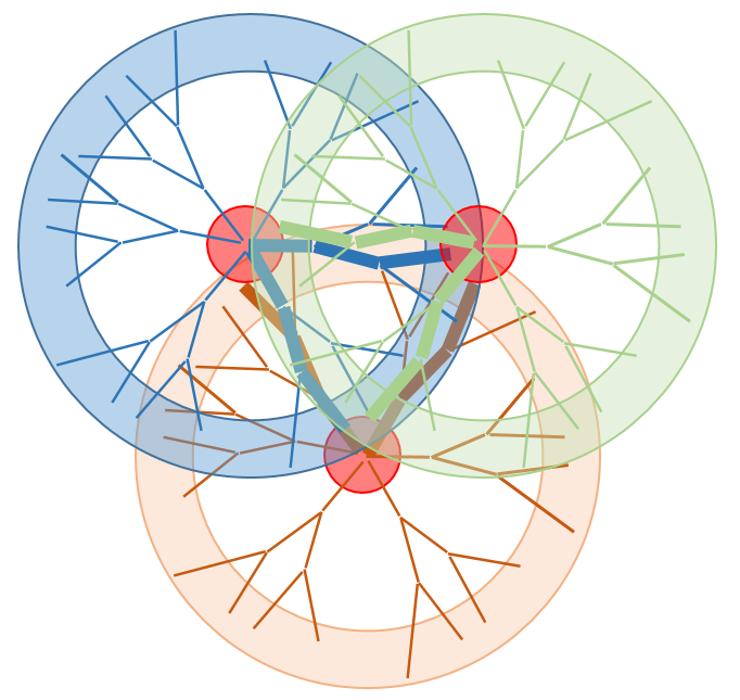
See below: Three hex-grid+temporal-sensing columns are sampling the imposed pattern in gold. As outlined above, these space-time puzzle pieces look for learned patterns and if it sees they it resonates with certain neighbors that also see the part of the pattern that they know. This activation pattern may spread to other groups of cells that are seeing parts of the same larger pattern.

When some pattern comes after this learning (babies are helpless until they learn something) each piece is trying to fit itself into the “picture on the box.” If it able to match up to one of its learned patterns it “snaps into place.” If enough of the pieces click together you can be said to have recognized the sensed pattern at that level. This pattern can be from outside the brain or from some region inside of the brain.
I come back to very basic theory as outlined in the “Why Neurons Have Thousands Of Synapses” paper.
Now consider these three dendrites apart from the rest of the dendrites in each cell.

Each has a sparse SDR that senses patterns – This paper suggests that the number of patterns that any individual segment of dendrites can hold is calculated as a relation of synapse sites and the percentage of active connections along that dendrite (no matter how you count it’s a huge number)
One of the issues mentioned in other posts is relating these dendrites into a larger pattern. SDR theory says that the odds of any of them misfiring with a pattern that is not a match are huge - what happens if these three are highly selective pattern matches are correlated by learning their own part of a larger pattern? In the case above, shown as gold activation fields. The learned pattern at each dendrite doesn’t have to match each other – only the part of the pattern they are learning by themselves. Each puzzle piece is a part of a larger puzzle; each becomes a peak of the mutual-reinforcing activity, a node in a hex-grid. This self-reinforcing property means that the chances of forming the wrong hex-grid from some larger pattern are small but there is a high probability that these sparse puzzle pieces will try to snap together.
The area of the hex-grid stretches as far as there are puzzle pieces matching the spatial-temporal pattern that is being applied to this area. The hex-grid forming properties sample the applied patterns (and surely there are more than one!) and sparsifies that into a new hex-grid.
We have the right facts on hand to estimate a ballpark number of hex-grids that can form in the human brain at the same time:
Column spacing ~= 0.03 mm
Hex-Grid spacing ~= .3 mm
Cortex area ~= 0.3 square meter
(300 mm / 0.3 mm)^2 = number of potential grid centers ~= 10 million simultaneous hex-grid sites.
… and how many patterns can be recognized at each hex-grid site:
Each 0.3 mm spaced grid hosts columns spaced at 0.03 mm, each is capable of being a nucleus of a grid location. Each individual column is capable of representing a large number of potential pieces but I will pick 300 to spitball a number.
(0.3 mm / 0.03 mm)^2 x 300 ~= 30000 code potential puzzle pieces in each grid location.
Someone with a better grasp of combinatorics than I can say how many overall things can be coded with 10 million letter positions with a 30000 letter alphabet but I recognize that it will be a staggeringly large number. This number shoots even higher if multiple hex-grids can co-exist in the same place at the same time.
These hex-grids work on the basic principles of attractors - applied patterns will recall the closest match. This recall process is a competitive process that fishes the best match out of a soup of possible matches, with a cooperative process between potential hex-grid locations to pick the best pattern that simultaneously satisfies both hex-grids recognition process.
For a superb visualization of hex-grids and how of hex-grids coding of different spatial scalings combine to represent a spatial location see this video by Matt Taylor.
THese hex-grid patterns are formed and projected to distant maps. There really would not be much point in just passing the pattern from map to map without any changes Two or more patterns have to project to a target map for some kind of local processing.
What kind of calculation can be performed when grids are combined?
The conjunction of hex-grid patterns has some extraordinary properties.
http://advances.sciencemag.org/content/1/11/e1500816.full
Let me share the juicy bits; looking at figure 2 to get a glimpse of the computing powers of hex-grids. We see the nodes of hex grids that have different phase/spacing/scaling (figures A & D) and the intersections of those hex-grids. In some places, these nodes line up and reinforce each other. (Figures B & C)

In pictures B & C we see various hex-grid fields representing Moser spatial grid locations with projections to the same areas by different spatial scaled grid size formations. Another way of saying this is checking for correlation in streams of space-time data. OK - just how do we get from a mishmash of the mixed-up signal to some sort of output that makes any sense at all?

In pictures A & D we see the combinations of various projections of some different scaled spatial grid patterns. Each color is from a different projecting area. What happens when these bits line up? That can form remarkably accurate points of local representation. Look back to the last pictures B & C - each of those clusters of blobs is doing this local recognition and summation. Weak peaks combine to make local clusters of strong peaks that drive the learning of this formation of and the future recognition of this correlation of patterns. (Figures A & D)
There is a regular transformation and grouping of these patterns as you move from map to map along the WHAT and WHERE streams. One of the common programming tasks is “parsing.” With a program that is working with a stream of words so it can be a bit harder to see that this is actually a general task that transcends the words. The brain is extracting meanings - patterns - things like syntax, semantics, sequences, and facts about the world. One stream is the WHAT of your perception and one stream is the WHERE of spatial components; how things are shaped or arranged. The process continues until you reach the temporal lobe. At that level what you are perceiving is your experience. This is all a passive process.
Since the usual programming process involves tokens like words it obscures the underlying process. Critters may not talk at all but they are surely doing much the same thing.
The little time/space puzzle pieces are much smaller units of meaning - small enough that it’s easy to miss the trees for the forest. Grouping of these little pieces combines to convey things about the world - some very small, some involving the entire brain map. There is not an exact match up to letters and words but it does help to convey the idea of fragments of meaning combining to parts of the meaning and so on.
Let me share how I see these maps being trained and the general principle of attractor representation.
First - what is an attractor?
If you think of the sea of columns with some pattern of activity impressed on it - how does this soup of learned patterns sort out the one matching or closest matching learned pattern? I see it as both a locally competitive and longer range cooperative process. Each column senses the overall pattern and if there is a match it starts to get a little excited. It’s firing rate goes up as it tries to resonate with the sensed pattern. Those cells that are sharing connections with other time-space puzzle pieces reinforce each other. As the cells get encouragement from other grid cells that are seeing parts that they also recognize the excitement grows. This mutual reinforcement gives the cells that are seeing part of an over-all pattern much more excitement than cells that just see a little bit that matches some prior learning.
The attractor part is that the sensed pattern reaches into the soup of codes and pulls out the matching learned pattern - as if the letters in a bowl of alphabet soup had a complete matching sentence swim up to the surface of the soup. It’s like a magnet draws the pattern (attracts it) out of the soup.
In the early stages, there is no ability to reason out why any pattern is special. As you learn it successive presentations “almost match” and get reinforced. The edges of the recognized pattern get refined as the cells on the edges of the recognized pattern encourage hex-grid cells that are on the fence to learn this pattern. I have to assume that the encouragement of mutual connections increases pattern learning due to the stronger excitement levels. Please recall that this is due to the recurring excitatory connections. As learning continue the learned pattern that is both sensed and projected becomes ever more detailed.
Going BIG!
Keep in mind that this is really interlocking patches of grids with bi-directional bundles of connections to other maps. I see good reasons to assume that mutual reinforcement of pattern recognition extends beyond an individual map to reach from map to map.
More in the next post in this series.
I’ve covered a huge swath of material here. If you have made it this far your head may be spinning trying sort out what bits go where in all this.
Let’s set everything in its place:
- The location of the columns that form the SDR processing nodes is fixed in space.
- An individual SDR can only reach as far as the dendrite arbor of a single neuron.
- The loops of axons that connect the columns in one map to the next are likewise fixed.
- The 0.5 mm range interconnections between neurons in the same area of the cortex is fixed.
- What the columns learn - using the proximal and distal dendrites - to recognize a bit of a spatial or temporal pattern, is what changes in this system. This learning is stored in learned connections/synapses along the proximal and distal dendrites. The SDRs. These change as learning progresses. The dendrites may also change and grow.
- These columns may interact with other columns via learned connections to organize into larger assemblies that take on the characteristics of hex-grids.
- The array of hex-grid cells is composed of columns that are individually matching parts of patterns using the learned SDRs.
The next post in the series focuses on combining these hex-grids into maps of information.
As always; I welcome your comments and ideas!

