Alternative sequence memory

That is a good analysis. I don’t personally see this as an indication that HTM is on the wrong path, though, since I believe brains suffer from the same problem. Suppose you as a human have learned a few sequences equally well, such that they are immediately recognizable to you. Also assume these are long sequences… I’m just showing a few letters of them:

…ABCDEFG…
…BCDEFAB…
…CDEFBCD…
…SEFCDEFS…

And then out of the blue, you unexpectedly start to hear “DEF…” (assume there is no other input providing context). There is no way you could tell me which of the above sequences is playing, but you would certainly expect that it is one of the five since you know them so well. As soon as the next letter comes in, you will immediately know which sequence you are in. My point is that even for a brain, it can take a few samples to clear up ambiguity when context has been lost.

I have experimented with several. One of the easier ones to visualize which would address this problem is based on logarithmic decay, something like the concept of eligibility traces from RL. The idea is that inputs that happen most recently would be more heavily represented than inputs which happened further back in time. Thus more cells representing “D after C after B after A” would be active than cells representing “S after F after V”, which would be more than the number of cells representing “B after A” and so-on. With a representation like that, one could tell that “VFS” happened after “AB” but before “CD”.

That’s super interesting. I came to somewhat a similar idea the other week (although from a different perspective) which I described in the original post under ‘Graded SDRs’ where a union of SDRs within an arbitrary time-window are ‘weighted’ depending on how recent they are. However that idea was replaced with bit-shifting because it avoids using graded SDRs while maintaining the use of binary SDRs and all the ordinary operations to process them. Though I find it interesting that you could quantify t+n of an SDR based on the number of cells representing it, I’ve not thought of that.

When you think of plugging into a hierarchy (theoretically – I haven’t actually tried it yet), you can imagine that this will impact which minicolumns win out during SP in the next higher level. You should be able to get a range of outputs that share different degrees of overlap, because the receptive fields of some minicolumns will favor a particular element in a sequence being more heavily represented, while other minicolumns will favor other elements of the sequence being more heavily represented.

I’ve been thinking about this TP issue and thought I’d try the other TP method we briefly discussed in another thread.

The code I use for the following examples can be found in this gist.

To see it in action check out this codepen

In the above gist I’ve written a network that does first-order-memory (layer 4) and temporal pooling (layer 3). I have used two sequences for demonstration - ABCD & XBCY. I have not implemented learning as I just want to demonstrate recall, so the weights are hard-coded. The symbols (XABCDY) are represented as single cells instead of SDRs for simplicity.

Layer 4 is simple as it just does first-order-memory. So A or X activates B, B activates C, C activates D and Y. All the weights in the matrix are binary, so the pre-synaptic neuron will activate the post-synaptic neuron instead of just depolarise/predict, I’ll explain why later. All the synapses between all the neurons in layer 3 are in the distal weight matrix.

Layer 3 has two cells to represent the two sequences. I have labelled them N & K. N represents ABCD, and K represents XBCY. While either sequence from layer 4 is playing out, the associated cell in layer 3 remains active. The synapses between layer 4 and 3 are in the proximal weight matrix. The weights are continuous. They simply represent the order in which the inputs arrive. For example, for N: A=4, B=3, C=2, D=1; for K: X:4, B=3, C=2, D=1. This simple encoding allows for competition between N & K during recall. If A was fed in from layer 4 then N will have a value of 4, and K will have a value of 0. Feed in B from layer 4, and feed back in the output from layer 3, then N will equal 43 and K will equal 3. The value for N is higher than K, and will remain that way for the duration of the sequence if C and D follow. I’ll explain later how layer 3 cells have their activation calculated.

The output from layer 3 is fed back into layer 4 through via the apical weights. By summing the inputs and weights from the distal and apical synapses the cell with the highest value is selected to be active. This again is based on the idea of competition. After C has been fed in, N will equal 432 and K will equal 32. C activates D & Y, but as D has apical synapses from N, D will have a value equal to N, while Y will have a value equal to K, so therefore D wins out.

The proximal synapses in layer 3 detect sequences in a specific order. A cell that represents a particular sequence from layer 4 will increase in value as the sequence plays out. For ABCD, N will increment like so: N=4, N=43, N=432, N=4321. If the sequence from layer 4 is incorrect the layer 3 cell will still increment, but just not as much. So for ACBD, N will increment like so: N=4, N=42, N=423, N=4231. For DCBA, N will increment: 1, 12, 123, 1234. The value of a cell in layer 3 is calculated: layer3[i] = layer3[i] * 10 + layer4[j]. So cells in layer 3 that have similar representations will have closer values than those with dissimilar representations.

In the code above I just input the beginning of the sequence (A or X) and let the memory unfold automatically over time. The in interesting thing is that if I input X, the layer 3 cell K has already predicted the whole sequence. The same for input A.

image

1 Like

Cool, I’ve been meaning to put together a test of this myself, but hadn’t gotten around to it. Of course the main deviation in your case is using the same cell for “B after A” and “B after X”, as well as “C after B after A” and “C after B after X”. It is interesting that having the pooling layer makes up for the ambiguity that this would normally lead to.

BTW, the order of the sequence inputting to K in your diagram is out of order (XYCB) :stuck_out_tongue_winking_eye:

21%20AM

10 Likes

Next step will be to add voting to further assist with solving ambiguity. For example, if I were to hear the melody “CCGGAAG”,

While looking at this, I would recognize the sequence as “Twinkle Twinkle”

but while looking at this, I would recognize it as the “ABC Song”
image

1 Like

Yup, also “D after C” and “Y after C”. When the temporal pooling layer (TP) sends biasing activation back to the temporal memory layer (TM), the TM layer only needs simple first-order-memory. This could be useful because it might be the case that the cells in the TP layer will be competing from top-down biasing from high-order regions.

The cells in the TP layer (N & K) have activity values which correspond to how similar the input sequence is compared to the sequence they represent. For the sequence ABCD, N has a value of 4321 and K a value of 32. To represent it as a vector [4321,32]. If the vector was to be squashed between 0 and 1 then we would get something like [1,0.5] (As N has a 100% similarity and K 50%). This could be thought of as a probability distribution (or a union of TP cells with different spike frequencies). In other words, instead of sending a single ‘name’ of the sequence to the region above (as represented [1,0]) it would send a probability of all ‘names’ of relevant sequences ([1,0.5]). This could be very useful information for the region above as it could combine probability distributions from bottom-up and top-down biases to help predict the next state in its own TM layer.

I’m not great at maths, but I think TP values ([4321,32]) should always be between 0 and 1, but I haven’t figured out how to calculate that while maintaining the increments based on sequence order.

The TP layer could also be sending concurrent sub-sequences like we were discussing before:

image
TP weight matrix

Lets add another TP cell Q which represents XABCDY. If the whole sequence XABCDY was fed into TP layer then Q will have the highest activation, N the second highest then K the least. This makes sense as Q is a perfect match while N(ABCD) is also a perfect match, but N is just a sub-sequence of Q, so therefore Q wins out. K is also a sub-sequence of Q but it is not as good of a match as N.

In my work i us a letter for chaos. Like “k”.

Example:

A, B, C are known.

AAAAkkkkkkAAAAkkkkkAAAA

Or:

ABCkABCk

k is unknown or will be know as the system learns more. But not known now.

1 Like

@Paul_Lamb I’m combining your explanations of TM bursting and the TP method we’ve been discussing before.

Sorry for such a long post!

It is known that SP is similar to SOMs in that it reduces the input space, so therefore ‘denoises’ the input, so therefore making it more stable. This is exactly what we want from a TP - in that it forms stable representations over similar inputs. In other words - it ‘generalises’.

A TP cell represents a sequence. The closer the input sequence is to the TP cell’s representation, the greater the TP cell’s activity. This is representative of the cell’s similarity to the input. Naturally most inputs will activate many cells at various levels. The cells with the greatest similarity will have the greatest activity. The cell with the greatest activity will inhibit the cells with lower activity causing a sparse representation of the feature that cell represents.

As discussed before, TP cells get input from column cells. So a TP cell’s potential pool is all the cells in the local columns. Using the same Hebbian learning as SP they learn the sequences of activated predicted cells in the columns. As you’ve visualised above, this looks like a union.

TP cells remain active while their input sequence plays out. Additionally, in this method they increase in activity for as long as they get input. When they lack input their activity drops.

image

Acceleration, the opposite of adaption

If a TP cell named Q represents the inputs ABCD, then when A is input then Q increases in activity. B is the next input so Q’s activity increases again. The next input is not C, so Q’s activity drops. The next input is also not C nor D so Q’s activity drops again. As Q was active for 50% of the inputs then you could say it was 50% similar to the input sequence. Any cells that had a higher similarity will have a greater activity, so in mutual inhibition they would have inhibited Q’s activity.

I will go over a few examples to demonstrate how this works with different sequences resembling some of the issues we faced in earlier posts.

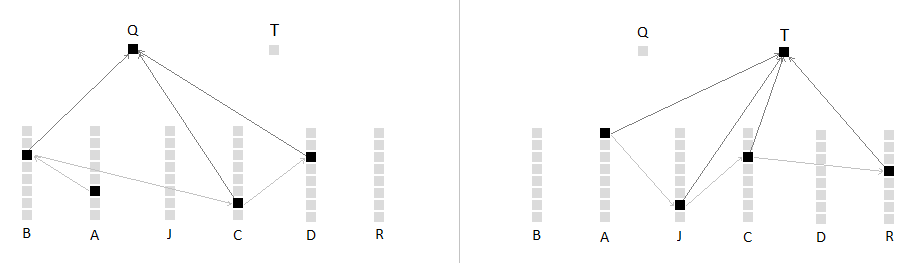
Lets say we have 6 columns for each symbol: B, A, J, C, D, R. We have 2 pooling cells: Q & T. Q represents the sequence ABCD, and T represents AJCR.

Sequence1: ABCDAJCR

This is a simple sequence because it is just a concatination of both sequences that the pooling cells represent. However it is a useful demonstration anyway.

1: Column A bursts and predicts cells in B and J columns. Pooling cells Q and T are equally activated. Because they are both activated they therefore inhibit each other, cancelling each other out.
2: The next input B activates the predicted cell in the B column so therefore activates the Q pooling cell. Q increases in activity while T remains silent from lack of input and from inhibition. Q is winning.
3: Input C will activate a predicted cell that B depolarised causing Q to increase in activity while T remains silent.
4: The same thing happens with input D.
5: Column A bursts and predicts cells in B and J columns. Pooling cells Q and T are equally activated. Due to mutual inhibition Q remains at the same level activity while T remains silent.
6: Input J activates its predicted column cell so therefore contributes activity to T. Q has no input and is inhibited by T, so therefore it looses much of its activity.
7: The same thing happens for input C, except now Q has no activity.
8: The same thing again with T being a clear winner.

This example can be graphed over time:

image

This shows the winning cell at each step:

image

So the fast changing sequence ABCDAJCR becomes more stable as the TP outputs QQQQJJJ. This output will in turn become more stable when pooled by the region above.

There is a slight problem. There is a mutual winner on J. Ideally T should be winning on J. So I suspect that activity changes are non-linear. But I’ll stick with linear examples for now.

Sequence 2: ABJCDR

This sequence is a blend of the two TP cell’s representations. We are jumping in and out of each.

1: Column A bursts and predicts cells in columns B & J. A also activates pooling cells Q & T but they mutually inhibit each other.
2: The next input B will activate the cell in column B and activate Q again. Q’s activity increases while T’s remains silent. Q is winning.
3: Next input J column will burst. This activates T while Q drops off. T is winning.
4: Input C activates the predicted cell in column C so therefore the pooling cell T. T is still winning. C did not activate Q because its column cell was not predicted.
5: Input D bursts and simply activates Q. As T did not get any input while receiving only inhibition from Q it will go back to being silent.
6: Input R bursts and simply activates T. T is winning.

The activity of Q and T can be graphed over the sequence:

image

The blue dots represent the winner at each moment of the sequence:

image

Q is active 40% of the time (ignoring the mutual inhibition in the first step) while T 60%. This means T is 20% more similar than Q is to the ABJCDR sequence. Of course this may not feel like that (as a human) reading these symbolic sequences. It is likely that is because we are already very familiar with ABCD and not familiar with AJCR. So this kind of suggests that pooling cells have weights (other than permanances) that increase over repetitions of stimuli. Or again top-down biasing can dramatically change the voting outcome.

The main advantage to this TP method is that a TP cell can represent an arbitrarily long sequence. As the sequence progresses the TP cell’s activity increases. This is probably biologically implausible as there are limits to a neuron’s frequency so it should only be able to represent a finite length sequence. But that’s only considering a single cell encoding, not a population encoding.

Anyway that’s the general idea. It’s all about the activity of the TP cell’s activity representing its similarity to the input sequence. I’ve realised there are many other ways to do this. But this is just one way of doing it with HTM’s TM. It has become clear to me tonight that of all the TM and TP methods I have explored (most of which were not posted in this thread) seem to all gravitate towards a core underlying idea. Some methods are more flexible than others. I’ll leave this here as I need to go to bed :slight_smile:

6 Likes

Very well described @sebjwallace.
It leads me to wonder:

  • How did TP cells ‘Q’ and ‘T’ come have those specific sets of TM cells in their receptive fields?
  • How do new TP cells come into existence? I’d think because no current cells are overlapping well with TM activity, but if there’s high bursting in TM due to high randomness in the inputs those sequences are kind of un-poolable right?

I’m reminded of how SP columns link to encoding bits, randomly at first and then learn by strengthening ties with those bits that help their overlap scores.
It seems TP cells may be doing something similar with TM cells, but over numerous time steps.

1 Like

After a few years… I remember I loved this thread. I don’t do anything like this now. But I remember how ecstatic I was working on this. Anyone still working on biologically-inspired AI - have fun - cuz it iz bruhh

2 Likes

Hi Sebastian, I’ve been working on biologically-inspired AI — HTM, precisely — to solve the problem of learning long-term dependencies in Continual and Embedded Reber Grammar. So, what do you mean by “it is bruhh”? :smile:
Just curious, since I’m using your idea on graded SDRs to solve the task.

Thanks!

1 Like

Biological sequence memory is still out for the jury as far as I can tell… although I’m still catching up on Numenta’s research. I have a fuzzy feeling that reference frames are similar to positional encodings in transformers. This allows for features to be relative to each other in time and space at various levels of framing. It’s the ‘structure’ of features, even repeated ones, i.e. AAAA or ABAB. They are positionally framed in reference to one another, as a fully connected graph. Very flexible and robust.

This may be of interest to you.

1 Like