koichi
April 19, 2018, 11:34am
1
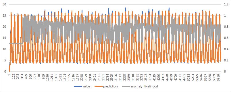
I have been working for anomaly detection using nupic and found that anomaly likelihood is always over 0.5.
Here is a typical example of anomaly likelihood result.
This result is calculated by using the program based on this. https://github.com/numenta/nupic/tree/master/examples/opf/clients/hotgym/anomaly/one_gym
Anomaly likelihood algorithm is found in this paper.
Real-Time Anomaly Detection for Streaming Analytics written by Subutai Ahmad and Scott Purdy.https://arxiv.org/pdf/1607.02480.pdf
Raw anomaly score is defined as:
Please note that ( 0 < St < 1)
Mean and variance are defined as follow:
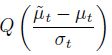
And then, the anomaly likelihood is defined as follows:
Q-function the Gaussian tail probability.
Gaussian destribution
0<
Since anomaly situation rarely happens,
As a result
That’s why nupic anomaly likelihood results are always over 0.5.
Does anyone have any comments on above discussion?
Kiochi showed me this in January, and I replcated it with hot gym:
I don’t think this is affecting anomaly likelihood functionality, but it would be good to figure out if he’s right about the cause of this.
So I asked for more details about this around the office and came up with a response.
The anomaly likelihood value never falls below 0.5 by design. We use 1.0 – Q(anomaly_scores – mean) as the anomaly likelihood. In our case, values far to the right or far to the left of the mean are both treated as being more anomalous. We handle this explicitly in the code:
def tailProbability(x, distributionParams):
"""
Given the normal distribution specified by the mean and standard deviation
in distributionParams, return the probability of getting samples further
from the mean. For values above the mean, this is the probability of getting
samples > x and for values below the mean, the probability of getting
samples < x. This is the Q-function: the tail probability of the normal distribution.


:param distributionParams: dict with 'mean' and 'stdev' of the distribution
"""
if "mean" not in distributionParams or "stdev" not in distributionParams:
  raise RuntimeError("Insufficient parameters to specify the distribution.")


if x < distributionParams["mean"]:
  # Gaussian is symmetrical around mean, so flip to get the tail probability
  xp = 2 * distributionParams["mean"] - x
  return tailProbability(xp, distributionParams)


# Calculate the Q function with the complementary error function, explained
# here: http://www.gaussianwaves.com/2012/07/q-function-and-error-functions
show original
With this understanding, the likelihood should never be smaller than 0.5 and it is enforced in the code.
koichi
April 20, 2018, 12:52am
4
Of course, I have check the code and the definition of anomaly likelihood which is defined in the paper has been implemented.
What I’ m pointing here is “Likelihood” is a technical term is statistics. For example, please refer to the following page.
In frequentist inference, a likelihood function (often simply the likelihood) is a function of the parameters of a statistical model, given specific observed data. Likelihood functions play a key role in frequentist inference, especially methods of estimating a parameter from a set of statistics. In informal contexts, "likelihood" is often used as a synonym for "probability". In mathematical statistics, the two terms have different meanings: Probability in this context describes the plausibility...
In actual deployment, we think the system should output anomaly likelihood so that users can change the threshold by themselves or give the threshold as a parameter. It’s really confusing for users who are familiar with statistics that likelihood is never smaller than 0.5. That’s also for me!!
I think nupic might use Q function incorrectly.
In statistics, the Q-function is the tail distribution function of the standard normal distribution. In other words,
Q
(
x
)
{\displaystyle Q(x)}
is the probability that a normal (Gaussian) random variable will obtain a value larger than
x
{\displaystyle x}
standard deviations. Equivalently,
Q
(
x
)
{\displaystyle Q(x If
...
Central limit theorem should be considered.
In probability theory, the central limit theorem (CLT) establishes that, in some situations, when independent random variables are added, their properly normalized sum tends toward a normal distribution (informally a "bell curve") even if the original variables themselves are not normally distributed. The theorem is a key concept in probability theory because it implies that probabilistic and statistical methods that work for normal distributions can be applicable to many problems involving othe...
1 Like


 > 0.5 and anomaly likelihood