It says in the paper that \hat{a}^{l} is a constant percentage of sparsity (value from 0 to 1). If initial d_{i}^{l}(t) is 1000 then it completely overwhelms the \hat{a}^{l} and we could as well remove it. What is the purpose of \hat{a}^{l} in this case or why is the value d_{i}^{l}(t) so overhelmingly big?
Aren’t you confusing a duty cycle value with the sliding window size?
I think they implemented boosting with moving average rather than sliding window in this paper.
Then, for active neurons it will gradually decrease and for inactive it will increase up until b_{i}^{l}(t)=e^{\beta \hat{a}^{l}} (since d_{i}^{l}(t) is positive by definition). In this case, it makes sense. I wonder why the actual value of \alpha was omitted in the paper, as it makes replication harder.
It might not make much of a difference but I think depending on the value of \beta , it may cause a floating point error because of the exponential function.
if the initial value of \ d_i^l(t)\ is \hat{a}^l\ , then e^{\beta(\hat{a}^l-d_i^l(t))} becomes 1 and the changing value of \ d_i^l(t)\ from now on would hardly cause the error.
EDIT: Actually, \hat{a}^l\ usually being really low, this wouldn’t be a problem at all. Sorry…
I guess a starting point would have to be if you understand what boosting is trying to do?
As I understand it, from a 10000 foot view, we have some cells that are strongly responding and hog up the response space. We have weaker cells that never reach firing potential so they never train on the inputs and learn any patterns.
In a relative sense we knock those stronger cells back and boost the weaker responding cells to allow them to train on the inputs and learn to respond.
The average term described is how many times a cell is fired over time, so a cell that fires one in ten cycles would average to 1/10. They reference a rolling average so the unit of time is some specified historical window. (the last 10 cycles in the example I just gave)
Over some period of time, we can compare the individual average values to find the very active units and the slackers - higher average values have been responding relatively more often. We can use these relative values to determine the ratio between winners and losers.
There is some “total amount of winning” and the portion that each cell receives of this total winning can be inversely distributed as a boost factor.
This co-factor (boost) for each cell that is combined with the normal output of the cell so that in the k-winner competion the cell seems to be responding more strongly. This will cause the cell to win more of the competitions and receive some training reinforcement.
As this weak cell wins more of the competitions the average winning stats will go up and it will receive a smaller boost, making room for weaker cells to be boosted.
I hope that this helps you parse the math and understand how it embodies this basic operation.
Thank you for providing the intuition, it roughly matches the intuition I got after reading the papers. However, your explanation doesn’t answer the questions I raised:
For the value of \alpha, unless you worked on the paper, you probably don’t know what value was used.
For the \alpha \cdot\left[i \in \text { topIndices }^{l}\right] you provided intuition but not the formula how that is calculated, and the paper doesn’t mention it. Set membership might return boolean in this case, and notation of a boolean in square brackets in an equation calculating real value output is not clear.
For the initial value of d_{i}^{l}(t), there is no mention either.
Lastly, code implementation that is published implements an older algorithm that doesn’t match Equation 6 in this paper.
I did some experimentation with the \alpha value. At the end of the day, it is an exponential moving average. I assumed:
initial value of d_{i}^{l}(t) is zero
a neuron fires with probability 0.7
[i \in \text { topIndices } l] is indicator function, meaning it is 1 if neuron fires, and 0 if not
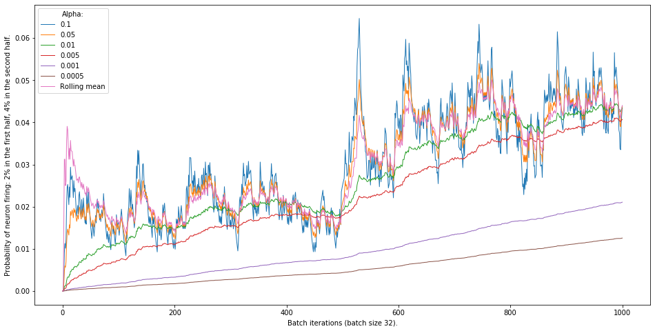
I plotted different values of duty cycle depending on \alpha, and this is what I got. On the vertical axis is the probability of the neuron firing at each iteration (fixed at 0.7), and on horizontal axis is the number of iterations:
This means that the duty cycle converges to the firing frequency and the value of \alpha determines:
how fast that happens
how much volatility if in the value of the duty cycle
Based on this, I think a good balance would be for \alpha to be in the range from 0.005 to 0.01.
You are correct, that is too high. In that original figure, I wanted to see how fast exponential average will converge to true underlying frequency of firing depending on the value of \alpha.
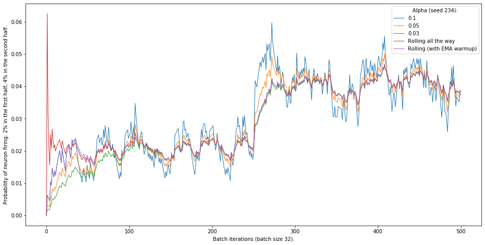
I made another figure, where the probability of firing is initially 2% (the one you provided as an example), then in the second half, it doubles. I wanted to examine how fast will the duty cycle catch up to “true” probability. I also implemented the duty cycle calculation using a rolling window average (as it is implemented in the original paper code). In addition, calculations are made in batches of size 32.
My conclusion is that initially, the rolling average can jump quite high for some neurons and stay relatively low for others. Another thing to note that the duty cycle will oscillate around the true firing frequency with quite some variance.
Update: I played some more and found that the optimal value of \alpha also depends on the batch size and so might be tricky to set up experimentally. Rolling mean implementation is much more stable (with the exception when at the beginning of training it is “warming up” and can look quite erratic.
If I may add, the most useful measure is - for the entire cell population - does the firing rate distribute the activation over the entire population of cells? Do all cells end up with some equal share of representation of the incoming stream of data? This question only applies in a fully connected network.
This question becomes more complicated with topology enabled as you care about equal representation in the neighborhood of the of the active areas. A topological based MNIST model would tend to have hot-spots of higher cell activity around the areas where digits tend to be presented - the center.
I suspect that the best display for this would be a heat map.
I agree that it is important to consider the whole population. Here I am only examining variability of the duty cycle values for a given neuron. The reasoning being to examine how stable it is given that probability of firing is fixed. If we extrapolate this to a whole population of neurons in a layer, and assume independency of firing rates between neurons (which is a good assumption at the beginning of training), then we can see that there will be quite some variability in the values of the duty cycle and boosting coefficients, meaning that some neurons will get boosted even though actually they all fire at the same rate.
The rolling window approach is especially unstable at the beginning of training, which will give a big boosted advantage to some of the neurons. To resolve this, I implemented exponential moving average at the beginning to “warm up” the duty cycle, and then it uses the rolling window average as it is implemented in the paper.
In the figure below notice how the red line (implementation as it is in the paper) is very unstable at the beginning, and the purple one, which uses exponential moving average for the first 1000 examples (around 32 batches) is much more stable.
that was perfect. Thank you very much for your kindness.
would you mind explain about the paper “how can we be so dense papers 'code” , what is the output of spatial pooling in this code ?
I run this code (how can we be so dense papers 'code) 2 days ago but it is not finished yet.I want to know why does it take so long ?what should I do to run this code faster?
You are not running HTM algorithms like the SP in the same way at all anymore. This paper is about applying ideas of HTM into today’s deep learning architectures. So at the core of this paper are DL networks, typically constructed to solve simple classification problems. These are compute heavy and take a long time to run. This is not like HTM at all. It is just an an attempt to add sparsity to the DL network in way that could benefit the system.
The sparsity is created with the k-winners activation step. If you don’t understand that, I suggest you need to learn about Deep Learning network architectures to understand this paper. I had to do the same thing. I recommend Andrew Ng’s Coursera course on Deep Learning.