Hi everyone. This time I also tried some visualizations.
First, meet the hex lattice
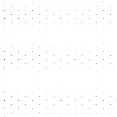
This here could very well be a top-down view of any cortical sheet model. Each microcolumn center would be identified with one of these points.
Each dot here has an equal spacing with any of its neighbors, and there are no ‘cornering’ neighbours distinct from ‘side’ neighbours, as would be the case with a square tiling scheme. I think it makes sense for an area so heavily concerned with topology as is V1. And in fact for any cortical area if we take the view that they all operate on same algorithm.
Now, we could object that using this weird layout seems to be lots of pain for little gain, however as shown below, there are very straightforward schemes to bind our common indexing for two-dimensional arrays to this:

You see that the grid above is still a common, regular, 2D addressable thing. Only skewed a little when representing it on display, or taking topology itself into account, so this layout has almost no impact on iteration times or global indexing complexity.
Now, an additional benefit is that any regular neighborhood is already a pretty good approximation of a circular area. Below is an illustration of an area which spans 4 neighbors from its center point, so this is a “9-across” area:

I have a quick and dirty Excel sheet at my side, which tells me that there are 61 distinct points inside this shape. And it will give me that number for any of the “neighbours from center” values. You can count them here if you wish.
With a few tweaks, you can fast-compute any offset-from the center (in the global addressing scheme described as a regular (x;y) index above) from any of these 0…60 possible address values. And this holds true at any scale, thus increasing the speed at which we can compute the extent, retrieve a point address, or iterate upon any of these roughly circular areas, of any diameter.
So, an index taken as an “offset-from-center” in the figure above would fit in only 6 bits. But obviously, from the reflection and estimations we carried around together with @bitking, we’d need to describe much larger areas for most of our concerns (which are both sides of the following matter : the extent of the axonal tree on one hand, and the dendritic extent on the other hand).
So let’s try to describe the “matter” in more detail.
You all know about the main excitatory cell of the cortical column : The pyramidal cell, and its HTM interpretation:

Let’s add some rulers around this one guy, or one of its close cousins…

Now that ~30µm for microcolumn-to-microcolumn center we settled on with @bitking is maybe not a figure everybody would agree on. It is on the lower end of the proposed scales from wikipedia (up to ~50 or even ~80µm). I believe however that, if one would take a greater figure than ~30µm, the philosophy of the proposed organization would not be much altered, and it would only reduce the count of stuff-per-area that we need to consider. So, ~30µm seems like the “worst case” scenario.
Each soma of a pyramidal cell is set on one microcolumnar index, on the hex layout. Typical horizontal dendritic extent (whether basal or apical) is at its ease in a 8-neighbourhood (17-across), but dendritic plasticity would allow them to grow up to a 12-neighborhood (25-across) if really information-starved. My Excell sheet tells me that there are 217 distinct possibilities for the ‘typical’ case, and up to 469 distinct possibilities when stretched. Those require at worse 9 bits to localize a subsegment relative to its cell’s soma position.

We can thus fully encode a 3D position for the subsegment on 16 bits, if we take 7 more bits for the vertical, giving us 128 possible “input template” per cortical area. Now what’s an input template ? It is a description of the axonal side of the problem. These subsegments, as exemplified by the little part magnified in the blue box two pics above, are highly localized. Beside allowing the finer 8-coincidency threshold detection I propose, this high specificity of localization is the whole point of them.
An “input template” is localized in the vertical axis of the receiving sheet, and may allow several “sources”. A source is : a “sheet” of origin (same or other cortical area, or even a deeper part of the brain such as LGN), and a specific “population” of cells within that sheet, sending axons towards the receiving area. Now, for each given source, there is in the model a precise topological relationship to the receiving area, which allow us to :
- define topologies as finely as the biological wiring we wish to simulate would require
- put an upper limit to the (otherwise huge) address of input cell, as viewed from a subsegment.
We’ll take a slice below to keep things simple in an example of topological mapping :

Maybe this looks like it is unecessarily complicated at this point, however now the wiring is completely specified. For a dendrite subsegment sampling the received input, the extent is applied the inverse scaling of the original mapping. In that example above, this would be divided by two, bringing the sampled neighbourood (around associated center) to two, ie. a 5-across area. You can check this on the above image, imagining how far apart on the source sheet could two cells having overlapping axonal arbors on the receiving sheet be situated. Any position in the original sheet layout thus gets a restricted area of incoming axonal overlap. For the (very lightweight) example above, it would look like this:

Now, the situation gets a little more complicated when the mapping is non-trivial, such as for ocular dominance stripes we have in V1, however I believe this is manageable.
Now, If we allow 12b or 13b per-synapse address, given a single sub-segment as proposed in my previous post, maybe there will be cases where the address-space is getting somewhat tight to allow multi-source with large axonal overlaps. Since I’m not confident we know of all weird-wiring cases which could potentially come up in the brain, let’s say we increase that value to a very conservative 16b per synapse… I’ll take whatever estimate you guys deem accurate for the max number of synapses in a subsegment having a length in the order of 40µm, but I believe this could be quite reasonable at this point.
At any rate, given a full-fledged ~6000 synapses cell, even with low filling-efficiency of subsegments at around 75% (this would bring the total synaptic “slot” count to ~8000), with 16b per synapse address and 4b for permanency value (permanency stored in another contiguous array, still very low profile as they’ll be stochastically updated), this makes the footprint of a cell at around 20KB.
The full connectivity state of a 100 thousand-cell simulation can thus be stored in around 2GB.
Seems high still ? Maybe. However the beauty of the topological structure is, no matter how many areas or minicolumns-per-area you’d wish to reasonably simulate, those 16b-address per synapse-on-given-subsegment values would never change. Were it computationally anywhere in reach, a full scale brain simulation could thus, in my view, still operate with those same values.
Which seems reasonable enough to start opening Visual Studio and work from there for the V1 sim. Now I have some work on my hands 