Help drawing HTM diagrams in LaTeX

[marty1885]

Hi all, I was busy finishing my graduation project. But I’m stucked at producing figures illustrating how Etaler utilizes multiple GPU/ use GPU and CPU together.

I came up with this code to produce a diagram for the TM w/ apical connections:

\tikzset{
	>=stealth',
	punktchain/.style={
		rectangle, 
		draw=black, very thick,
		text width=4.5em, 
		minimum height=3em, 
		text centered, 
		node distance=3cm},
	line/.style={draw, thick, <-},
	every join/.style={->, thick,shorten >=1pt},
	decoration={brace},
	tuborg/.style={decorate},
	tubnode/.style={midway, right=2pt},
}

\begin{figure}[H]
\begin{center}
\begin{tikzpicture}
[node distance=.8cm,
start chain=auto]
	\node[punktchain] (sp1) {Spatial Pooler};
	\node[punktchain, below of=sp1] (tm1) {Temporal Memory};
	\node[punktchain, right of=tm1] (sp2) {Spatial Pooler};
	
	%%FIXME: Why is the direction reversed?
	\path [line] (tm1) -> (sp1);
	\path [line] (tm1) -> (sp2);
\end{tikzpicture}
\caption{Example use of multiple backends}
\label{gph_many_backend:figure}
\end{center}
\end{figure}

Which produces this figure:

And I want to make it look like so (edited using mspaint, you get the idea)

I have tried several ways to produce the graph, but none of my solutions work. Any help is very appreciated.

Thanks.

[CollinsEM]

When I need a simple diagram for a LaTeX document, I typically write a PostScript file. It’s really not that hard and it’s pretty flexible. It has semantics like SVG. Just Google PostScript tutorial. I may post a couple of helpful links here later after I get a chance to check my bookmarks.

[CollinsEM]

Then again, about 15 minutes noodling around in InkScape, and I made this.

InkScape is free, and can export to just about any file type you need (including LaTeX with PSTricks macros).

[marty1885]

Hmm… I never thought I can do that. Thanks!

[Jonathan_Mackenzie]

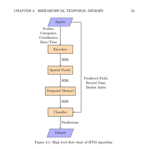
I used Tikz in my thesis, here’s my diagram of the basic htm process:

\usepackage{tikz}
\usetikzlibrary{shapes.geometric, arrows,automata,positioning}
\tikzstyle{startstop} = [rectangle, rounded corners, minimum width=3cm, minimum height=1cm,text centered, draw=black, fill=red!30]
\tikzstyle{io} = [trapezium, trapezium left angle=70, trapezium right angle=110, minimum width=3cm, minimum height=1cm, text centered, draw=black, fill=blue!30]
\tikzstyle{process} = [rectangle, minimum width=3cm, minimum height=1cm, text centered, draw=black, fill=orange!30]
\tikzstyle{decision} = [diamond, minimum width=3cm, minimum height=1cm, text centered, draw=black, fill=green!30]
\tikzstyle{arrow} = [thick,->,>=stealth]


HTM at a high level has 4 main steps (see \autoref{fig:htm}) \citep{Hawkins2016}:
\begin{figure}[ht!]
	\centering
	\begin{tikzpicture}[node distance=2.5cm]
		\node(start) [io]{Inputs};
		\node(enc)[process, below of=start, yshift=-0.75cm]{Encoders};
		\node(sp)[process, below of=enc]{Spatial Pooler};
		\node(tm)[process, below of=sp]{Temporal Memory};
		\node(clac)[process, below of=tm]{Classifier};
		\node(out) [io, below of=clac]{Output};
		\node(side)[right of=start, inner sep=0,minimum size=0,draw=none, fill=none]{};
		\draw[arrow] (start) -- node[anchor=east, text width=6em, text centered] {Scalars, Categories, Coordinates, Date/Time}(enc);
		\draw[arrow] (enc) -- node[anchor=west] {SDR}(sp);
		\draw[arrow] (sp) -- node[anchor=west] {SDR} (tm);
		\draw (start) -- (side);
		\draw[arrow] (side) |- node[anchor=west, text width=8em, text centered,yshift=3.5cm]{Predicted Field, Record Num, Bucket Index} (clac);
		\draw[arrow] (tm) -- node[anchor=west] {SDR} (clac);
		\draw[arrow] (clac) -- node[anchor=west]{Predictions}  (out); 
	\end{tikzpicture}
	\caption{High level flow chart of HTM algorithm \label{fig:htm}}
\end{figure}

Gives you